library(ggplot2)
library(rnaturalearth)
library(sf)
library(ggtext)
library(showtext)

#add font awesome
font_add('fa-brands', here::here('fonts/fa-brands-400.ttf'))
showtext_auto()

library(dplyr)Ukraine: The Center of Europe
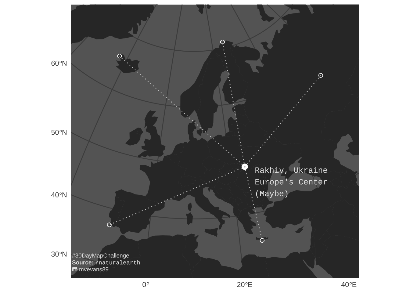
Day 5 of the #30DayMapChallenge - Ukraine
Today’s challenge is a map about Ukraine. I learned recently that there is a point in Ukraine considered the geographic midpoint of Europe. Then, I did some research today and learned this is a highly debated topic, not least of which because the definition of ‘Europe’ really depends on who you talk to. But I was already committed to the idea. For this, I manually georeferenced some points that seemed to be on the edge of Europe, at least to this non-European currently residing in Europe. I then plotted it over a basemap from the rnaturalearth package and used the sf package to add some lines.
#download basemap of the world
world.map <- ne_countries(scale = 110, returnclass = 'sf') %>%
st_transform(crs = 3035)
#identify center
center <- data.frame(lon = 23.833, lat = 48.5) %>%
st_as_sf(coords = c("lon", "lat"), crs = 4326) %>%
#transform to do in meters
st_transform(3035)
#identify edges
n <- data.frame(lat = 71.095089, lon = 25.783898) %>%
st_as_sf(coords = c("lon", "lat"), crs = 4326) %>%
#transform to do in meters
st_transform(3035) %>%
mutate(position = "North")
sw <- data.frame(lat = 37.033281, lon = -8.918422) %>%
st_as_sf(coords = c("lon", "lat"), crs = 4326) %>%
#transform to do in meters
st_transform(3035) %>%
mutate(position = "Southwest")
se <- data.frame(lat = 34.928006, lon = 24.857155) %>%
st_as_sf(coords = c("lon", "lat"), crs = 4326) %>%
#transform to do in meters
st_transform(3035) %>%
mutate(position = "Southeast")
nw <- data.frame(lat = 65.852065, lon = -23.589617) %>%
st_as_sf(coords = c("lon", "lat"), crs = 4326) %>%
#transform to do in meters
st_transform(3035) %>%
mutate(position = "Northwest")
e <- data.frame(lat = 57.880922, lon = 56.307665) %>%
st_as_sf(coords = c("lon", "lat"), crs = 4326) %>%
#transform to do in meters
st_transform(3035) %>%
mutate(position = "East")
edges <- bind_rows(n, sw, se, nw, e)
map.bbox <- st_bbox(st_buffer(edges, 5e5))
#create distance lines
dist.lines <- st_sfc(mapply(function(a,b){st_cast(st_union(a,b),"LINESTRING")}, center$geometry, edges$geometry, SIMPLIFY=FALSE)) %>%
st_as_sf(crs = 3035) %>%
mutate(length_km = round(st_length(.)/1e3))
#define caption for easier reading
caption.lab <- paste0("#30DayMapChallenge<br>",
"<b>Source: </b><span style='font-family:mono;'>rnaturalearth</span><br>",
"<span style='font-family:fa-brands;'></span> mvevans89")
ggplot() +
geom_sf(data = world.map, fill = "gray20", color = NA, size = 0.6) +
geom_sf(data = center, color = "white", size = 3) +
geom_sf(data = dist.lines, color = "gray80", linetype = 21) +
geom_sf(data = edges, color = "white", size = 2, shape = 21) +
coord_sf(xlim = map.bbox[c(1,3)], ylim = map.bbox[c(2,4)]) +
annotate(x = st_coordinates(center)[1]+2e5, y = st_coordinates(center)[2]-3e5,
geom = "text", label = "Rakhiv, Ukraine\nEurope's Center\n(Maybe)",
color = "gray90", hjust = 0, size = 3.5, family = "mono") +
geom_richtext(data = data.frame(x = map.bbox[c(1)] - 3e5,
y = map.bbox[c(2)] + 5e4),
aes(x = x, y = y, label = caption.lab), fill = NA, label.color = NA,
color = "gray90", size = 2.5, hjust = 0) +
theme(panel.background = element_rect(fill = "gray40"),
panel.grid.major = element_line(color = "gray30"),
# axis.text = element_blank(),
axis.title = element_blank(),
axis.ticks = element_blank())